2. Extraction of a large time series of meteorological variables

2.1 Requirements

library(rgee)
library(sf)  
library(tidyverse)
library(lubridate)
ee_Initialize()

── rgee 1.1.2.9000 ──────────────── earthengine-api 0.1.297 ── 
 ✓ user: not_defined
 ✓ Initializing Google Earth Engine:  DONE!
 ✓ Earth Engine account: users/antonybarja8 
────────────────────────────────────────────────────────────── 

3.2 Reading vector layer of study area

lima <- st_read(
  "https://github.com/healthinnovation/sdb-gpkg/raw/main/Lima_provincia.gpkg",
  quiet = TRUE) %>%
  summarise()

2.3 Transformation of sf object to a feature collection

lima_ee <-  lima %>% 
  sf_as_ee()

2.4 Processing data with rgee

terraclim <-  ee$ImageCollection$Dataset$IDAHO_EPSCOR_TERRACLIMATE$
  select(c("tmmx","pr"))$
  filterDate("1990-01-01","2021-12-31")$
  toBands()
# Extracting data
lima_data <- ee_extract(
  x = terraclim,
  y = lima_ee,
  fun = ee$Reducer$mean(),
  sf = FALSE)

2.5 Processing data for mapping

lima_temp <- lima_data %>% as_tibble() %>% 
  mutate(region = "LIMA") %>% 
  pivot_longer(X199001_pr:X202012_tmmx) %>% 
  separate(col = name,into = c("date","variable"),sep = "_") %>% 
  mutate(date = ym(gsub("X","",date))) %>% 
  separate(col = date,into = c("year","month"),sep = "-") %>% 
  mutate(month = factor(month,labels = month.abb))

2.6 Time series plot - Lima

# Maximum temperature
lima_temp %>% 
  pivot_wider(names_from = variable,
              values_from = value) %>% 
  mutate(date = ymd(paste(year, month, "01", sep = "/"))) %>%
  ggplot(aes(x = date, y = tmmx, col = tmmx)) +
  geom_line() + 
  scale_x_date(date_breaks = "6 months", 
               date_minor_breaks = "6 months",
               date_labels = "%B %Y") +
  scale_color_viridis_c(option = "magma") +
  theme_minimal() +
  theme(axis.text.x = element_text(angle = 90, vjust = 0.5, hjust=1),
        legend.position = "top")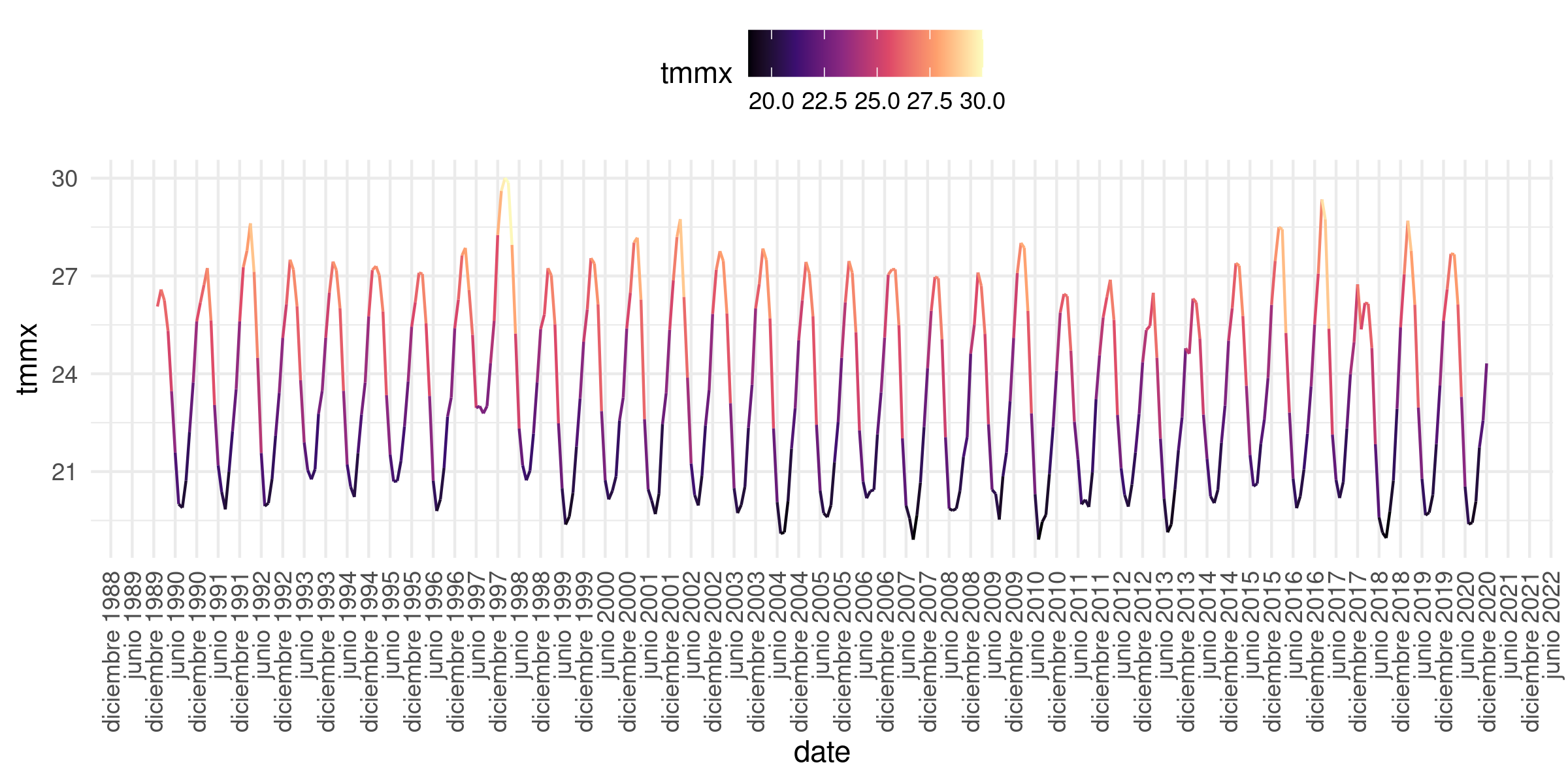

2.7 Time series plot for the 24 departaments of Peru

# Reading vector layer
dep <- st_read(
  "https://github.com/healthinnovation/sdb-gpkg/raw/main/departamentos.gpkg",
  quiet = TRUE) %>% 
  dplyr::select(NOMBDEP)

# Time estimate ~ 12 min
dep_list <- list()
for(i in 1:nrow(dep)){
  dep_ee <- dep[i,] %>% sf_as_ee()
  pet <- ee_extract(
    x = terraclim,
    y = dep_ee,
    fun = ee$Reducer$mean(),
    sf = FALSE)
  dep_list[[i]] <- pet
}

# Processing data for mapping 
dep_pet <- dep_list %>% 
  map_df(.f = as_tibble) %>% 
  pivot_longer(X199001_pr:X202012_tmmx) %>% 
  mutate(variables = gsub("[^prtmmx]", "", name) ,
         date = gsub("\\D", "", name) %>% as.integer()) %>% 
  mutate(value = case_when(
    variables =="pr" ~ value,
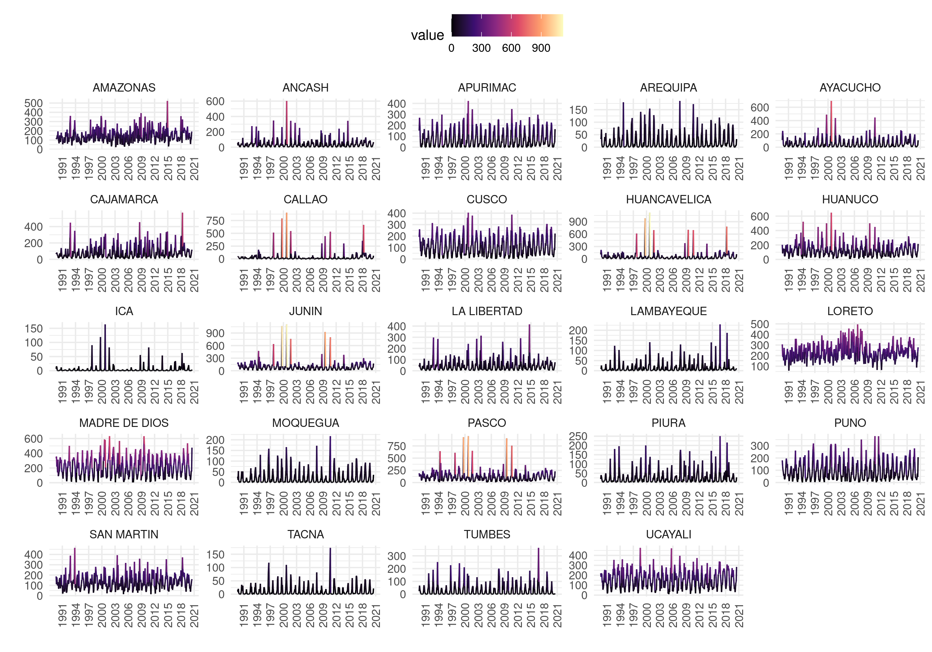
    variables == "tmmx" ~ value *0.1))

# Accumulated precipitation
dep_pet  %>% 
  mutate(date = ymd(sprintf("%s01",date))) %>%
  filter(variables == "pr") %>% 
  ggplot(aes(x = date, y = value, col = value)) +
  geom_line() + 
  scale_x_date(date_breaks = "36 months", 
               date_minor_breaks = "36 months",
               date_labels = "%Y") +
  scale_color_viridis_c(option = "magma") +
  theme_minimal() +
  theme(axis.text.x = element_text(angle = 90, vjust = 0.5, hjust=1),
        legend.position = "top") +
  facet_wrap(~NOMBDEP,ncol = 5 , scale = "free") + 
  labs(x = "" , y = "")